Premise

While human’s are decent at estimating human age based on physical appearance, it’s relatively easy to fool the eyes. Visuals are inherently malleable, and humans have become very good at altering their physical appearance to achieve a desired effect, be it to look younger or older.

Determined to never be fooled again, lets build an AI to perform this task at a more biological level!

Brainstorming

First we must beg the question: what biological data inputs are available for predicting someone’s age? If you read the title, you probably know the direction i’m going in: human blood. A first thought might be to make use of DNA, but the problem is that DNA is mostly static throughout the course of a person’s life, and therefore wouldn’t lend itself very well to our goal.

However, what can be taken from the blood and changes throughout the course of a person’s life? DNA Methylation!

What is DNA Methyation?

For those of you unfamiliar with it, DNA methylation is a biological phenomenon by which methyl groups are added to certain positions in the traditional DNA molecule; it can be thought of as adding a 5th base to standard DNA, where the 5th base is able to change back and fourth with cytosine (one of the four DNA bases) throughout the course of your life.

The biological significance is gene activation. All the cells in your body have the same DNA, but obviously they do different things. DNA methylation is what accounts for this discrepancy; it tells a cell which genes to turn on or off. Added bonus is that it’s easy to ask someone on the spot for their DNA Methylation profile in reponse to being asked to guess their age (that’s a joke).

Gathering Resources

Now that we have found the input for the model, DNA methylation, and the output, age, we need to find the actual datasets we will use to build our AI model.

While DNA methylation can be extracted from blood samples using DNA methylation sequencers, it may prove costly; the sequencing machine costs $900,000, not to mention an additional $375 per sample. The good news is that NIH released a dataset with 732 presequenced samples, along with their ages which range from 14 to 94 years old!

All that’s left to do now is actually write the code.

Preprocessing

Once downloading the datasets and beginning data visualization to get a feel for what we would be working with, we realize we have a bit of a problem: the methylation sequencer spits out a whopping 476,366 features per sample, each of which is a value between 0 and 1.

 1
 2
 3
 4
 5
 6
 7
 8
 9
10
11
12
13
14
15

    # Get dataset. It's is too big to come as a single file
    !wget -O "./GSE87571_Matrix_Avg_Beta.txt.gz" "https://www.ncbi.nlm.nih.gov/geo/download/?acc=GSE87571&format=file&file=GSE87571%5Fmatrix1of2%2Etxt%2Egz"
    !wget -O "./GSE87571_Matrix_Avg_Beta2.txt.gz" "https://www.ncbi.nlm.nih.gov/geo/download/?acc=GSE87571&format=file&file=GSE87571%5Fmatrix2of2%2Etxt%2Egz

    # Extract dataset
    !gunzip "./GSE87571_Matrix_Avg_Beta.txt.gz"
    !gunzip "./GSE87571_Matrix_Avg_Beta2.txt.gz

    # Merge data set files into one
    !cut -d$'\t' -f1 --complement "./GSE87571_Matrix_Avg_Beta2.txt" > newFile && mv newFile "./GSE87571_Matrix_Avg_Beta2.txt"
    !paste "GSE87571_Matrix_Avg_Beta.txt" "./GSE87571_Matrix_Avg_Beta2.txt" > matrix.csv

    # Remove every other column because every other column has blank values
    !awk '{{printf "%s ", $1}for(i=2;i<=NF;i=i+2){printf "%s ", $i}{printf "%s", RS}}' matrix.csv > final_matrix.cs
    

How is DNA Methylation Quantified?

In order to understand what these features represent, we must quickly digress into a bit of biology. Each of these 470,000+ corresponds to a single cytosine position in the human genome (we don’t get a response from every single position). You may have expected the value to be either 0 or 1 because a position either is or is not methylated within a single cell, however this is not the case. Reason being that rather than passing the sequencer a single cell, it is passed thousands of cells, each of which may have variable DNA methylation. If 80% of these cells were methylated at position 637,293 of the genome, for example, then the value of the feature corresponding to the 637,293 position of the genome would be 0.8.

Dimension Reduction Time

Back to the computer science: 470,000+ features sounds nice at first, but is a recipe for overfitting when we only have 700 samples at our disposal. Such is the curse of dimensionality. A better approach is to first filter down the features before performing any machine learning. We do so by selecting only the 25 features (25 is relatively arbitrary) that have the highest correlation with age. It’s important to note that we must first split the dataset into training and testing sets at a ratio of 9:1 in order to prevent data contamination. i.e. if the features were to be selected based on information from the test set, then the model would become biased.

 1
 2
 3
 4
 5
 6
 7
 8
 9
10
11
12
13
14

# Split data
train_annotated, test_annotated = train_test_split(data_annotated, test_size=0.10)

# Calculate correlation matrix
corr_array = []
for col in train_annotated.columns:
  corr_array.append(train_annotated[col].corr(train_annotated["Age"]))

print(len(corr_array))
corr_df = pd.DataFrame(corr_array, columns=["Correlation"], index=train_annotated.columns)

corr_df["Abs_Corr"] = corr_df.Correlation.abs()
corr_df.sort_values("Abs_Corr", inplace=True, ascending=False)
print(corr_df.head(26))

After filtering the features we visualize them with the heatmap below. The y-axis represents the selected methylation positions, while the x-axis represents the samples sorted in ascending order by age for the train and test sets respectively. The colors encode a methylation value between 0 and 1, where black corresponds to 0% methylation and white corresponds to 100% methyation.

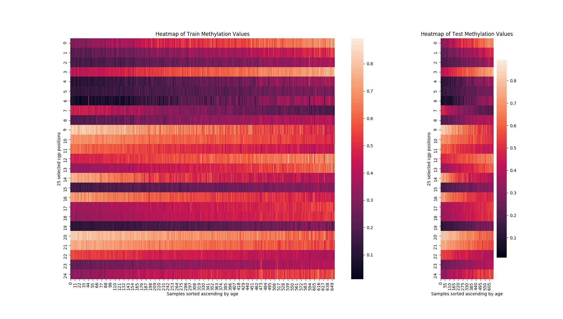
The training data looks wonderful, with distinct colors trends for each of the features implying strong correlation with age. You can see that as age increases from left to right, the methylation values trend monotonically in one direction or the other; these are the types of signals in the data that machine learning can make use of. The test set’s data trends were not quite as clear, but this is to be expected because the filtering of the features is based on the training set, not the test set. However, the horizontal trends are still strong enough to get excited about.

Training The Model

Now that the hardest part of machine learning is over (preprocessing), it is time to actually train a model. We can deploy a pretty basic 3 layered neural net. It includes three dense layers each with 1024 ReLU nodes, three dropout layers each with a rate of 0.2, and a final dense layer with a single node corresponding to the predicted age. Lets train it for 50 epochs on a loss function of mean squared error. Let me know if you are able to find a better model!

 1
 2
 3
 4
 5
 6
 7
 8
 9
10
11
12
13
14

# Basic neural net with 4 dense layers
model = tf.keras.models.Sequential([
    tf.keras.layers.Dense(1024, activation='relu', input_shape=(25,)),
    tf.keras.layers.Dropout(0.2),
    tf.keras.layers.Dense(1024, activation='relu'),
    tf.keras.layers.Dropout(0.2),
    tf.keras.layers.Dense(1024, activation='relu'),
    tf.keras.layers.Dropout(0.2),
    tf.keras.layers.Dense(1)
])

model.compile(loss= "mean_squared_error" , optimizer="adam", metrics=["mean_squared_error"])
model.summary()
model.fit(train_processed_np, train_processed_ages,  epochs=50, validation_data=(test_processed_np, test_processed_ages)

Results

Now it’s finally time to answer the big question. How well can we predict age using just the DNA methylation extracted from a blood sample? Take a look at the chart below and see for yourself:

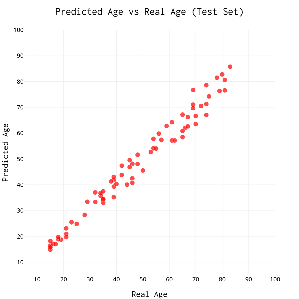
When comparing the model’s predictions with the actual ages of the samples, we find a mean absolute deviation of 3.19 and standard error of the estimate of 0.46. All predicted ages are within ±10 years of real age; over 70% are within ±5 years of real. This is something to get excited about! Next time we are asked to guess someone’s age, we can be confident to answer within about 3 years on average :)

Building A User Interface

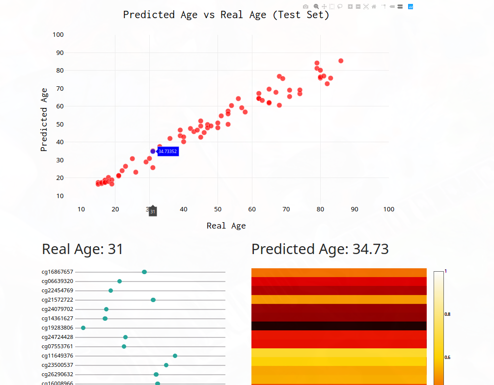
You can’t truly enjoy a machine learning model without a good user interface, so let’s build one that would allow anyone to play with the different features and see how predicted age changes. All we have to download the model weights, import plotly, add some sliders, and boom! A nice user interface. See it for yourself at https://epigenosys.com! Github

Conclusion

I hope you enjoyed. Make sure to check out https://epigenosys.com to play with the model yourself. See all the code here. Watch the associated YouTube video here

Thanks to Simon Berens for reading drafts of this